Tuning hyperparameters for random forests

Tl;dr

• Random forests are great as baseline models, better than GBDTs like xgboost/ lightgbm/ catboost.
• The other side of the coin: don’t expect a lot of improvement from tuning random forests.
• When tuning hyperparameters, choose at least one to explore bagging, one to explore subspace sampling, and one (preferably two) to control model complexity.
• Most papers on this have flaws. This essay is an interim report on the WIP benchmark we are doing.

Are Random Forests still relevant?

In A Comparative Analysis of XGBoost¹, the authors analyzed the gains from doing hyperparameter tuning on 28 datasets (classification tasks). scikit-learn’s RandomForestClassifier, with default hyperparameter values, * did better than xgboost models (default hyperparameter values) in 17/28 datasets (61%)², and * did better than tuned xgboost models (trained on 3840 hyperparameter configurations) in 9/28 datasets (32%)³.

¹ Bentéjac, Candice, Anna Csörgő, and Gonzalo Martínez-Muñoz. “A Comparative Analysis of XGBoost.” arXiv preprint arXiv:1911.01914 (2019).

² Table 3 in[^1], a cleaned-up version can be found here

³ Table 3 in[^1], a cleaned-up version can be found here

⁴ page 19, https://www.kaggle.com/kaggle-survey-2020

Random forests are great baseline models - it’s hard to train a poorly performing random forest. With xgboost/ lightgbm/ catboost, you not only have to tune more hyperparameters to get good results, but you also have to tune the number of trees in the ensemble, adding a lot of runtime to your experiments (you barely have to tune the number of trees in a random forest). There is a reason why random forests are more popular than more-advanced GBDT and variants (as implemented in xgboost/ lightgbm/ catboost)⁴.

So while GBDTs are great for kaggle competitions, random forests are an integral part of the practising data scientist’s toolbox.

Why this essay?

Random forests have a reputation for not being very tunable: while the default values of hyperparameters will often produce a good enough random forest, on the downside tuning a lot of parameters does not produce a lot of improvements in model performance.

The typical implementation of random forests has too many parameters for us to tune all of them together, and the gain from doing so is not expected to be significant anyway. In the wild, we see all sorts of subsets of the hyperparameters being tuned, without much empirical sense behind it.

We haven’t found any concise overview of best practices for tuning hyperparameters for random forests, so we wrote one. If you know of such a guide, please let us know @dataBiryani. Besides, we wanted to run our own experiments to validate the papers we read. Some of those experiments are included in the accompanying repo⁵.

⁵ https://github.com/soumendra/principled-hp-tuning-tree-based-ensembles

Random forest hyperparameters: some intuitions

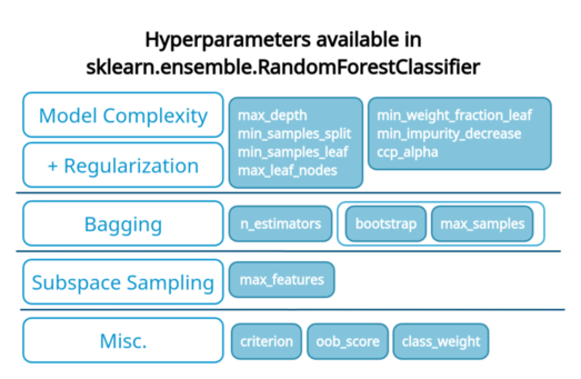
Before jumping into details, we’ll put some structure into how we think about the hyperparameters found in random forest implementations. Those hyperparameters typically relate to one of the following aspects of training an RF:

• Bootstrapping (bagging)
• Subspace sampling
• Base-model complexity and regularization

To understand where this comes from, let’s quickly review how random forests are constructed.

How random forests work

Random forests are collections of independently-constructed decision trees. Here is how we construct those individual trees:

1. Create a bootstrapped sample: We create a subset of all available observations by repeatedly sampling one observation at a time, typically with replacement.
2. Train the decision tree
   • subspace sampling at every node: Every time we need to split a node in the decision tree, we consider only a subset of the features (subspace sample) from the bootstrapped sample (instead of all features).
   • control Base-model complexity and prevent overfitting with regularization: To maximize the ensemble performance, we must make the right choice in bias/variance trade-off. Decision trees offer a lot of hyperparameters to control the bias/variance trade-off by manipulating the complexity and size of the base learners generated. Bootstrapping and subspace sampling parameters contribute to this as well, but we consider them separately. Also, most hyperparameters manipulating base-model complexity have some amount of regularisation effects.
3. Aggregate the trees: For a given observation, we create an ensemble prediction by taking the predictions from individual trees and taking the mode (classification) or averaging the values (regression). The earlier bootstrapping, followed by this aggregating, is called bagging.

Hyperparameters of random forest

In this essay, we’ll look at the implementation of random forests in sklearn (RandomForestClassifier, RandomForestRegressor).

Hyperparameters for Random Forest

How should we tune the hyperparameters?

We propose that instead of tuning a mish-mash of hyperparameters, we tune some hyperparameters from each of the groups we listed above: Bootstrapping (bagging), Subspace sampling, and Base-model complexity/regularization.

In the following sections, we go a little deeper into how we should choose hyperparameters from each of those three groups.

The experiment

We looked at a few research papers to find meta-experiments around hyperparameter tuning of random forests. However, we came up short because of a few reasons.

1. The tuning is done only for small datasets, which we felt was not representative of the kind of models that are trained in practice today.
2. It was hard to reproduce the experiments. Some involved hard-to-obtain datasets, and in some cases a few datasets have been lost.
3. We wanted to look deeper into the model tuning - not only the score and hyperparameter-configuration of the top model but of a few more models at the top.
4. We believed better tuning was needed to draw fairer conclusions. Sometimes not the right subsets were tuned, sometimes not enough tuning was done (too few configurations), and sometimes the values chosen were rather extreme for the given datasets!

So we started our own benchmarking exercise, the code and output of which is available at https://github.com/soumendra/principled-hp-tuning-tree-based-ensembles/tree/main/random_forest/. It is still a work in progress. We started with the smallest datasets in the openml-cc18 benchmark⁶ and so far have added 41 datasets to our benchmark. More details can be found in the repo.

⁶ https://docs.openml.org/benchmark/#openml-cc18

⁷ https://github.com/soumendra/principled-hp-tuning-tree-based-ensembles/blob/main/random_forest/output/openml_experiments.csv

The summary of the dataset and the results is available here⁷.

Bootstrapping/Bagging

n_estimators

While n_estimators, the number of trees in the ensemble, is critical to the success of the random forest, it is also the easiest to tune - simply set it to a large enough number.

In his Random forests⁸ paper, Breiman proved that generalization errors for classification and regression random forests converge as the number of trees grows. Moreover, in the paper To tune or note to tune the number of trees in random forest⁹, the authors provide theoretical and empirical validity to the monotonicity of the performance measure curve for a combination of tasks and performance metrics (e.g., logloss for classification). It follows that the measure will keep improving as we increase the number of trees, eventually leveling off.

⁸ Breiman, Leo. “Random forests.” Machine learning 45.1 (2001): 5-32.

⁹ Probst, Philipp, and Anne-Laure Boulesteix. “To tune or not to tune the number of trees in random forest.” The Journal of Machine Learning Research 18.1 (2017): 6673-6690.

For certain kinds of smallish datasets for specific combinations of tasks and performance metrics (e.g., AUC for classification), they find that the monotonicity doesn’t hold, and very specific non-monotonous patterns are exhibited (as can be seen below).

Should we tune the number of trees?

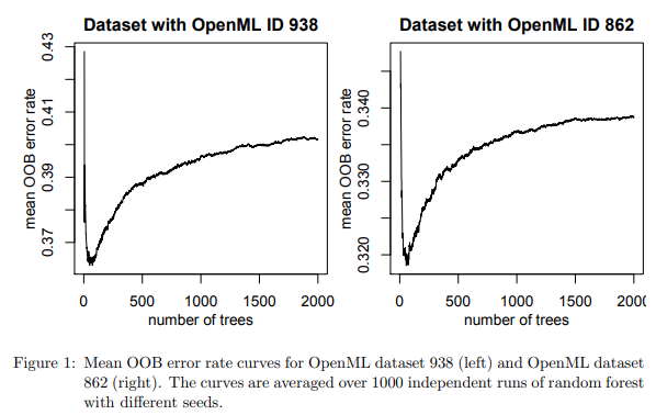
In these cases (about 10% of the datasets they analyzed), the error rate curves, after reaching their lowest values, gradually rise again as the number of trees grows, eventually to converge at a value very slightly higher than the lowest value achieved before. Quoting from the paper:

the curve grows again after reaching its lowest value, leading to a value at 2000 trees that is by at least 0.005 bigger than the lowest value of the OOB error rate curve for T \in [10, 150].

Using math and empirical analysis, they describe the kind of small datasets exhibiting this behaviour, where chasing this kind of minuscule improvement in model performance is perhaps not very meaningful given the associated computational costs.

In practice, we should set n_estimators to a computationally feasible large number and not spend time tuning it.

parallel coordinates plot of top 5 models from 500

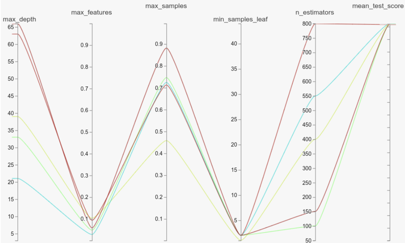
The parallel coordinates plot above shows the top 5 models from the 500 trained on the ‘mfeat-factors’ dataset that has the highest number of datapoints (#samples x #features) among the 41 datasets in the benchmark. As we can see, there is a model with just 100 trees almost matching the top-performing model. The story remains the same when we consider other datasets with high (electricity, optdigits) or low (balance-scale, ilpd) number of data points.

bootstrap

If bootstrap is False, the whole dataset is used to build the trees (no bagging), significantly taking away our ability to make an effective bias-variance trade-off. We almost never have to tune this.

max_samples

With n_estimators and bootstrap not providing many opportunities for tuning, max_samples (default value of 1.0) is the only hyperparameter left that we can use to tune bagging. We again turn to parallel coordinate plots for some empirical guidance.

If we look at electricity, high values of max_samples seem to be effective (all hyperparameters seem to be in a stable region as well). This is not a lot of value-add though, as the default value is 1.

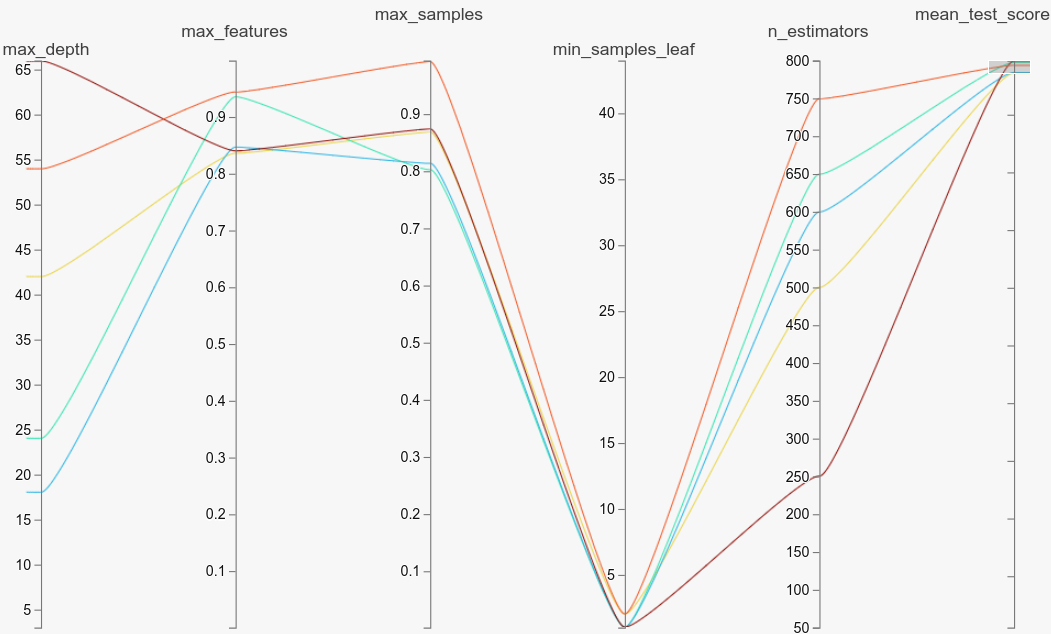
parallel coordinate plots for electricity

On the other hand, if we look at balance-scale, low values of max_samples seem to be effective. Tuning the parameter here was very valuable, as most of the top models have low values of max_samples (far from the default value of 1).

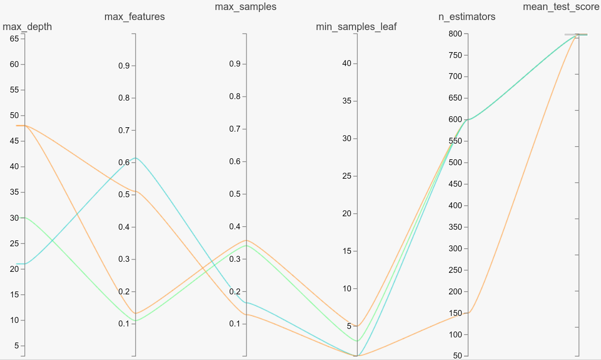
parallel coordinate plots for balance-scale

You can look at the other plots we linked to above, or play with any of the datasets using the notebook in the repo to see that it makes sense to tune max_samples well.

If computational power is not a bottleneck, you can simply tune it with RandomSearchCV. Otherwise, you may use a combination of GridSearchCV and RandomSearchCV (optional, you may stick to GridSearchCV) to perform a greedy hill-climb (use a small grid to identify promising areas and refine the grid in iterations).

Subspace sampling

max_features

scikit-learn’s RandomForestClassifier and RandomForestRegressor provide only one hyperparameter to tune subspace sampling - max_features.

Let’s look at parallel coordinate plots for electricity and mfeat-factors.

The electricity dataset has 8 features, so the default value of max_features is 8**0.5/8 (sqrt(n_features)/n_features) ~ 0.35. Looking at the parallel coordinates plot for electricity, we see that high values of max_features (between 0.65 to 0.95) seem to be effective (all hyperparameters seem to be in a stable region as well). So tuning max_features was very valuable here.

parallel coordinate plots for electricity

If we look at mfeat-factors, low values of max_features seem to be effective. The default value is 216**0.5/216 (sqrt(n_features)/n_features) ~ 0.07 and most of those values center around that (you can look at the exact values by running the notebook). We don’t seem to have gained much by tuning the parameter here.

parallel coordinate plots for mfeat-factors

If you inspect other datasets, you’ll find that the default value (or something close to it) is lurking somewhere there in the top-10 to top-30 models, and in general, we gain in performance by tuning this parameter.

Since this is the only parameter controlling subspace sampling, we should ideally tune it.

Base model complexity and regularization

Controlling the size of the tree

1. max_depth: The maximum depth to which the trees will be expanded (by splitting).
2. min_samples_split: If the number of training samples at a node is less than this, a split will not happen.
3. min_samples_leaf: A split at a node will happen only if it leaves min_samples_split number of training samples in resulting nodes.
4. max_leaf_nodes: A leaf node in a decision tree is where decisions happen (all training samples reaching this node are assigned to a specific class). This parameter specifies the maximum number of leaf nodes allowed.
5. min_impurity_decrease: In a decision tree, a node is split when a criteria (using a feature) is found that best reduces impurity. If this value is set (default 0), a node is split only if the decrease in impurity is greater than or equal to this value.

max_depth is the most direct way of controlling the size of the decision trees being trained (and thus its bias/variance), and is a popular choice for tuning.

When tuning hyperparameters, we should pick up at least one (ideally at least two) of these hyperparameters to ensure that we are exploring enough variations in the model complexity.

min_samples_split and min_samples_leaf control model complexity very similarly, and it doesn’t make a lot of empirical sense to tune them together (except if you are choosing values in different ranges for them - min_samples_split in [1, 2, 5, 7] and min_samples_leaf in [1, 10, 20]. That said, if our parallel coordinate plots are anything to go by, we should perhaps explore these parameters minimally. The interval [1, 5] seems to be a good enough solution. We haven’t benchmarked larger datasets in our experiment, but we don’t expect this to change.

parallel coordinate plots for mfeat-factors - low values of min_samples_leaf produce the best models

GridSearch vs RandomSearch vs Bayesian/evolutionary/others

Unless you are severely constrained by computing resources and have some hypothesis about what the values of your preferred hyperparameters should be, random search is almost always a better idea compared to grid search. The paper Random search for hyper-parameter optimization¹⁰ provides compelling empirical evidence in favor of random search.

¹⁰ Bergstra, James, and Yoshua Bengio. “Random search for hyper-parameter optimization.” The Journal of Machine Learning Research 13.1 (2012): 281-305.

We’ll explore other methods of tuning the hyperparameters (with benchmarks) in future essays.